Overview

Dates and times are abundant in data and essential for answering questions that start with when, how long, or how often. However, they can be tricky, as they come in a variety of formats and can behave in unintuitive ways. This article teaches you the essentials of parsing, manipulating, and computing with dates and times in R. By the end, we’ll have mastered the lubridate package, a member of the tidyverse, specifically designed to handle dates and times. we’ll also have applied the new skills to explore how often R versions are released, when the weather is good in Auckland (the birthplace of R), and how long monarchs ruled in Britain.

Libraries

library(readr)
library(anytime)
library(ggplot2)
library(dplyr)
library(lubridate)
library(ggridges)
library(fasttime)
library(tidyverse)
library(microbenchmark)

Warning message:
"package 'microbenchmark' was built under R version 3.6.3"

install.packages("microbenchmark")

package 'microbenchmark' successfully unpacked and MD5 sums checked

The downloaded binary packages are in
    C:\Users\user\AppData\Local\Temp\RtmpUtbNCC\downloaded_packages

Dates and Times in R

R doesn’t know something is a date or time unless you tell it. We’ll explore some of the ways R stores dates and times by exploring how often R versions are released, and how quickly people download them.

Introduction to dates

Dates

Different conventions in different places

27th Feb 2013

NZ: 27/2/2013

USA: 2/27/2013

The global standard numeric date format

{% fn 1%}

ISO 8601 YYYY-MM-DD

Values ordered from the largest to smallest unit of time

Each has a xed number of digits, must be padded with leadingzeros

Either, no separators for computers, or - in dates

1st of January 2011 -> 2011-01-01

Dates in R - Packages that importd ates:readr,anytime

2003-02-27

1974

as.Date("2003-02-27")

2003-02-27

"2003-02-27"

'2003-02-27'

str("2003-02-27")

 chr "2003-02-27"

str(as.Date("2003-02-27"))

 Date[1:1], format: "2003-02-27"

Specifying dates

R doesn’t know something is a date unless you tell it. If you have a character string that represents a date in the ISO 8601 standard you can turn it into a Date using the as.Date() function. Just pass the character string (or a vector of character strings) as the first argument.

We’ll convert a character string representation of a date to a Date object.

# The date R 3.0.0 was released
x <- "2013-04-03"

# Examine structure of x
str(x)

# Use as.Date() to interpret x as a date
x_date <- as.Date(x)

# Examine structure of x_date
str(x_date)

# Store April 10 2014 as a Date
april_10_2014 <- as.Date("2014-04-10")
april_10_2014

 chr "2013-04-03"
 Date[1:1], format: "2013-04-03"

2014-04-10

Automatic import

Sometimes we’ll need to input a couple of dates by hand using as.Date() but it’s much more common to have a column of dates in a data file.

Some functions that read in data will automatically recognize and parse dates in a variety of formats. In particular the import functions, like read_csv(), in the readr package will recognize dates in a few common formats.

There is also the anytime() function in the anytime package whose sole goal is to automatically parse strings as dates regardless of the format.

# Use read_csv() to import rversions.csv
releases <- read_csv('datasets/rversions.csv')

# Examine the structure of the date column
str(releases$date)

# Various ways of writing Sep 10 2009
sep_10_2009 <- c("September 10 2009", "2009-09-10", "10 Sep 2009", "09-10-2009")

# Use anytime() to parse sep_10_2009
anytime(sep_10_2009)

Parsed with column specification:
cols(
  major = col_double(),
  minor = col_double(),
  patch = col_double(),
  date = col_date(format = ""),
  datetime = col_datetime(format = ""),
  time = col_time(format = ""),
  type = col_character()
)

 Date[1:105], format: "1997-12-04" "1997-12-21" "1998-01-10" "1998-03-14" "1998-05-02" ...

[1] "2009-09-10 EAT" "2009-09-10 EAT" "2009-09-10 EAT" "2009-09-10 EAT"

Why use dates?

Dates act like numbers

Date objects are stored as days since 1970-01-01

as.Date("2020-07-13") > as.Date("2020-01-01")

TRUE

as.Date("2020-07-10") + 3

2020-07-13

as.Date("2020-07-13") - as.Date("2019-07-13")

Time difference of 366 days

Plotting with dates

first_days = c(as.Date("2020-01-01"), as.Date("2020-02-01"), 
               as.Date("2020-03-01"), as.Date("2020-04-01"), 
               as.Date("2020-05-01"), as.Date("2020-06-01"), 
               as.Date("2020-07-01"), as.Date("2020-08-01"))
plot(first_days, 1:8)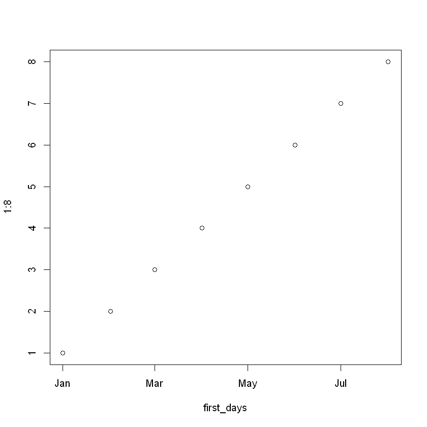

ggplot() + geom_point(aes(x=first_days, y=1:8))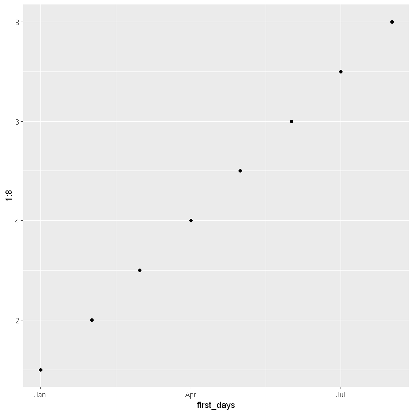

R releases

head(releases)

minor	patch	date	datetime	time	type
60	NA	1997-12-04	1997-12-04 08:47:58	08:47:58	patch
61	NA	1997-12-21	1997-12-21 13:09:22	13:09:22	minor
61	1	1998-01-10	1998-01-10 00:31:55	00:31:55	patch
61	2	1998-03-14	1998-03-14 19:25:55	19:25:55	patch
61	3	1998-05-02	1998-05-02 07:58:17	07:58:17	patch
62	NA	1998-06-14	1998-06-14 12:56:20	12:56:20	minor

Plotting

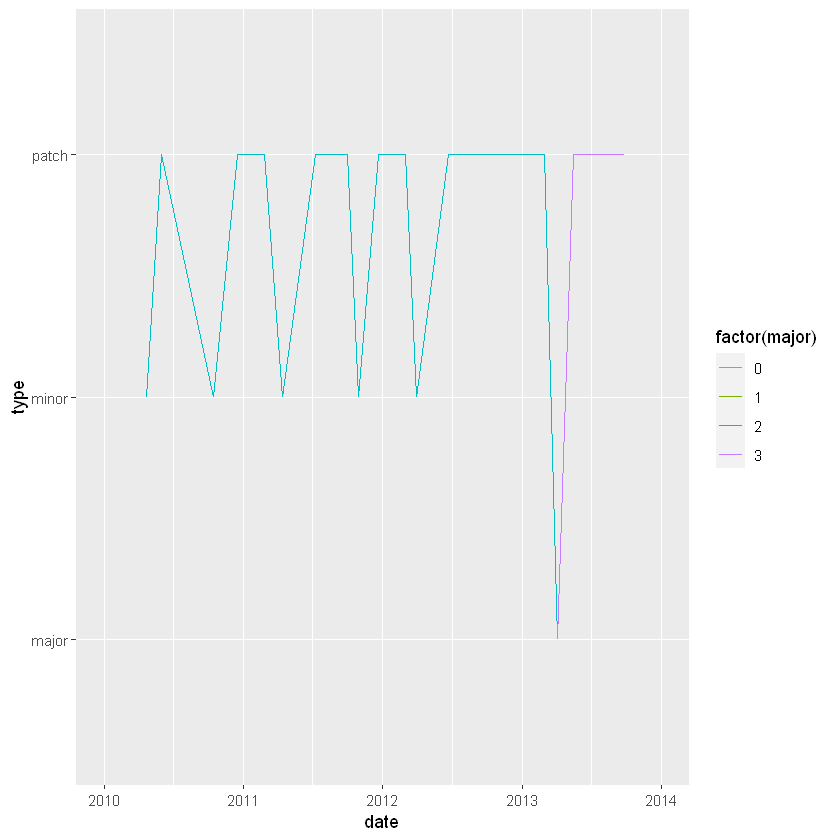
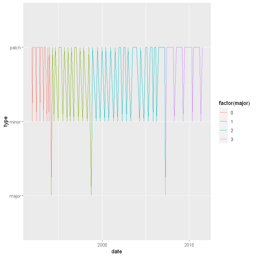
If you plot a Date on the axis of a plot, you expect the dates to be in calendar order, and that’s exactly what happens with plot() or ggplot().

We’ll make some plots with the R version releases data using ggplot2. There are two big differences when a Date is on an axis:

If you specify limits they must be Date objects.
To control the behavior of the scale we’ll use the scale_x_date() function.

# Set the x axis to the date column
ggplot(releases, aes(x = date, y = type)) +
  geom_line(aes(group = 1, color = factor(major)))

# Limit the axis to between 2010-01-01 and 2014-01-01
ggplot(releases, aes(x = date, y = type)) +
  geom_line(aes(group = 1, color = factor(major))) +
  xlim(as.Date("2010-01-01"), as.Date("2014-01-01"))

# Specify breaks every ten years and labels with "%Y"
ggplot(releases, aes(x = date, y = type)) +
  geom_line(aes(group = 1, color = factor(major))) +
  scale_x_date(date_breaks = "10 years", date_labels = "%Y")

Warning message:
"Removed 87 row(s) containing missing values (geom_path)."

Arithmetic and logical operators

Since Date objects are internally represented as the number of days since 1970-01-01 we can do basic math and comparisons with dates. We can compare dates with the usual logical operators (<, ==, > etc.), find extremes with min() and max(), and even subtract two dates to find out the time between them.

# Find the largest date
last_release_date <- max(releases$date)

# Filter row for last release
last_release <- filter(releases, date==last_release_date)

# Print last_release
last_release

# How long since last release?
Sys.Date() - last_release_date

major	minor	patch	date	datetime	time	type
3	4	1	2017-06-30	2017-06-30 07:04:11	07:04:11	patch

Time difference of 1110 days

Sys.date()- in the code, it simply returns today’s date.

What about times?

ISO 8601

HH:MM:SS

Largest unit to smallest

Fixed digits

Hours: 00 – 24

Minutes: 00 – 59

Seconds: 00 – 60 (60 only for leap seconds)

No separator or :

Datetimes in R

Two objects types:

POSIXlt - list with named components

POSIXct - seconds since 1970-01-01 00:00:00

POSIXct will go in a data frame

as.POSIXct() turns a string into a POSIXct object

str(as.POSIXct("1997-06-15 00:01:00"))

 POSIXct[1:1], format: "1997-06-15 00:01:00"

Timezones

"2013-02-27T18:00:00"-6pm localtime

"2013-02-27T18:00:00Z"-6pm UTC

"2013-02-27T18:00:00-08:00"-6pmin Oregon

as.POSIXct("1997-06-15T18:00:59Z")

[1] "1997-06-15 EAT"

as.POSIXct("1997-06-15T18:00:59Z", tz="UTC")

[1] "1997-06-15 UTC"

Datetimes behave nicely too

Once a POSIXct object,datetimes can be:

Compared

Subtracted

Plotted

Getting datetimes into R

Just like dates without times, if you want R to recognize a string as a datetime you need to convert it, although now you use as.POSIXct(). as.POSIXct() expects strings to be in the format YYYY-MM-DD HH:MM:SS.

The only tricky thing is that times will be interpreted in local time based on your machine’s set up. You can check your timezone with Sys.timezone(). If you want the time to be interpreted in a different timezone, you just set the tz argument of as.POSIXct().

Sys.timezone()

'Africa/Nairobi'

# Use as.POSIXct to enter the datetime 
as.POSIXct("2010-10-01 12:12:00")

# Use as.POSIXct again but set the timezone to `"America/Los_Angeles"`
as.POSIXct("2010-10-01 12:12:00", tz = "America/Los_Angeles")

# Examine structure of datetime column
str(releases$datetime)

[1] "2010-10-01 12:12:00 EAT"

[1] "2010-10-01 12:12:00 PDT"

 POSIXct[1:105], format: "1997-12-04 08:47:58" "1997-12-21 13:09:22" "1998-01-10 00:31:55" ...

Datetimes behave nicely too

Just like Date objects, you can plot and do math with POSIXct objects. We’ll see how quickly people download new versions of R, by examining the download logs from the RStudio CRAN mirror. R 3.2.0 was released at “2015-04-16 07:13:33” so cran-logs_2015-04-17.csv contains a random sample of downloads on the 16th, 17th and 18th.

# Import "cran-logs_2015-04-17.csv" with read_csv()
logs <- read_csv("datasets/cran-logs_2015-04-17.csv")

# Print logs
head(logs)

Parsed with column specification:
cols(
  datetime = col_datetime(format = ""),
  r_version = col_character(),
  country = col_character()
)

datetime	r_version	country
2015-04-16 22:40:19	3.1.3	CO
2015-04-16 09:11:04	3.1.3	GB
2015-04-16 17:12:37	3.1.3	DE
2015-04-18 12:34:43	3.2.0	GB
2015-04-16 04:49:18	3.1.3	PE
2015-04-16 06:40:44	3.1.3	TW

# Store the release time as a POSIXct object
release_time <- as.POSIXct("2015-04-16 07:13:33", tz = "UTC")

# When is the first download of 3.2.0?
logs %>% 
  filter(datetime==release_time,
    r_version == "3.2.0")

# Examine histograms of downloads by version
ggplot(logs, aes(x = datetime)) +
  geom_histogram() +
  geom_vline(aes(xintercept = as.numeric(release_time)))+
  facet_wrap(~ r_version, ncol = 1)

datetime	r_version	country

`stat_bin()` using `bins = 30`. Pick better value with `binwidth`.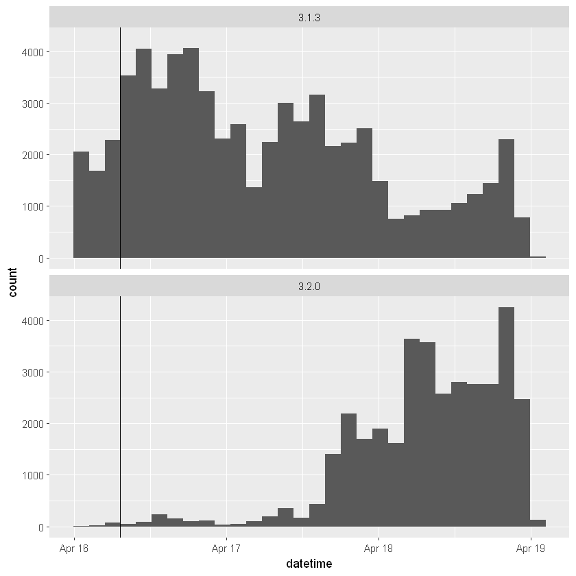

it takes about two days for downloads of the new version (3.2.0) to overtake downloads of the old version (3.1.3)

Why lubridate?

lubridate

Make working with dates and times in R easy!

tidyverse package

Plays nicely with builtin datetime objects

Designed for humans not computers

Plays nicely with other tidyverse packages

Consistent behaviour regardless of underlying object

Parsing a wide range of formats

ymd("1997-06-15")

1997-06-15

dmy("15/06/97")

1997-06-15

parse_date_time(c("June 15th, 1997", "15th June, 1997"), order=c("mdy", "dmy"))

[1] "1997-06-15 UTC" "1997-06-15 UTC"

Manipulating datetimes

akl_daily = read_csv("datasets/akl_weather_daily.csv")
head(akl_daily)

Parsed with column specification:
cols(
  date = col_character(),
  max_temp = col_double(),
  min_temp = col_double(),
  mean_temp = col_double(),
  mean_rh = col_double(),
  events = col_character(),
  cloud_cover = col_double()
)

date	max_temp	min_temp	mean_temp	mean_rh	events	cloud_cover
2007-9-1	60	51	56	75	NA	4
2007-9-2	60	53	56	82	Rain	4
2007-9-3	57	51	54	78	NA	6
2007-9-4	64	50	57	80	Rain	6
2007-9-5	53	48	50	90	Rain	7
2007-9-6	57	42	50	69	NA	1

akl_daily_m <- akl_daily %>%
    mutate(
        year = year(date),
        yday = yday(date),
        month = month(date, label=TRUE)
    )
head(akl_daily_m)

date	max_temp	min_temp	mean_temp	mean_rh	events	cloud_cover	year	yday	month
2007-9-1	60	51	56	75	NA	4	2007	244	Sep
2007-9-2	60	53	56	82	Rain	4	2007	245	Sep
2007-9-3	57	51	54	78	NA	6	2007	246	Sep
2007-9-4	64	50	57	80	Rain	6	2007	247	Sep
2007-9-5	53	48	50	90	Rain	7	2007	248	Sep
2007-9-6	57	42	50	69	NA	1	2007	249	Sep

Other lubridate features

Handling timezones

Fast parsing of standard formats

Outputting datetimes

Parsing and Manipulating Dates and Times with lubridate

Dates and times come in a huge assortment of formats, so the first hurdle is often to parse the format you have into an R datetime. We will explore how to import dates and times with the lubridate package. We’ll also explore how to extract parts of a datetime. We’ll practice by exploring the weather in R’s birthplace, Auckland NZ.

Parsing dates with lubridate

ymd()

27th of February 2013

ymd() - year, then month, then day

ymd("1997-06-15")

1997-06-15

ymd("97/6/15")

1997-06-15

ymd("97t6t15")

1997-06-15

Friends of ymd()

ymd(),ydm(),mdy(),myd(),dmy(),dym(), dmy_hm()

parse_date_time(x = ___, order = ___)

Formatting characters

Character Meaning Character Meaning

d numeric day of the month a Abbreviated weekday

m month of the year A Full weekday

y Year with century b Abbreviated month name

Y year without century B full month name

H hours (24 hours) I hours (12 hour)

M minutes P AM/PM

z Timezone, offset

Character	Meaning	Character	Meaning
`d`	numeric day of the month	`a`	Abbreviated weekday
`m`	month of the year	`A`	Full weekday
`y`	Year with century	`b`	Abbreviated month name
`Y`	year without century	`B`	full month name
`H`	hours (24 hours)	`I`	hours (12 hour)
`M`	minutes	`P`	AM/PM
`z`	Timezone, offset

Selecting the right parsing function

lubridate provides a set of functions for parsing dates of a known order. For example, ymd() will parse dates with year first, followed by month and then day. The parsing is flexible, for example, it will parse the m whether it is numeric (e.g. 9 or 09), a full month name (e.g. September), or an abbreviated month name (e.g. Sep).

All the functions with y, m and d in any order exist. If the dates have times as well, you can use the functions that start with ymd, dmy, mdy or ydm and are followed by any of _h, _hm or _hms.

# Parse x 
x <- "2010 September 20th" # 2010-09-20
ymd(x)

# Parse y 
y <- "02.01.2010"  # 2010-01-02
dmy(y)

# Parse z 
z <- "Sep, 12th 2010 14:00"  # 2010-09-12T14:00
mdy_hm(z)

2010-09-20

2010-01-02

[1] "2010-09-12 14:00:00 UTC"

Specifying an order with `parse_date_time()`

What about if you have something in a really weird order like dym_msh?There’s no named function just for that order, but that is where parse_date_time() comes in. parse_date_time() takes an additional argument, orders, where you can specify the order of the components in the date.

For example, to parse "2010 September 20th" you could say parse_date_time("2010 September 20th", orders = "ymd") and that would be equivalent to using the ymd() function from the previous exercise.

One advantage of parse_date_time() is that you can use more format characters. For example, you can specify weekday names with A, I for 12 hour time, am/pm indicators with p and many others. Another big advantage is that you can specify a vector of orders, and that allows parsing of dates where multiple formats might be used.

# Specify an order string to parse x
x <- "Monday June 1st 2010 at 4pm"
parse_date_time(x, orders = "ABdyIp")

# Specify order to include both "mdy" and "dmy"
two_orders <- c("October 7, 2001", "October 13, 2002", "April 13, 2003", 
  "17 April 2005", "23 April 2017")
parse_date_time(two_orders, orders = c("Bdy", "Bdy", "Bdy", "dBy", "dBy"))

# Specify order to include "dOmY", "OmY" and "Y"
short_dates <- c("11 December 1282", "May 1372", "1253")
parse_date_time(short_dates, orders = c("d0mY", "0mY", "Y"))

[1] "2010-06-01 16:00:00 UTC"

[1] "2001-10-07 UTC" "2002-10-13 UTC" "2003-04-13 UTC" "2005-04-17 UTC"
[5] "2017-04-23 UTC"

[1] "1282-12-11 UTC" "1372-05-01 UTC" "1253-01-01 UTC"

Note

when a date component is missing, it’s just set to 1? For example, the input 1253 resulted in the date 1253-01-01.

Weather in Auckland

make_date(year, month, day)

make_date(year=1997, month=6, day=15)

1997-06-15

make_datetime(year, month, day, hour, min, sec) for datetimes

dplyr Review

mutate() - add new columns (or overwrite old ones)

filter() - subset rows

select() - subset columns

arrange() - order rows

summarise() - summarise rows

group_by() - useful in conjuction with summarise()

Import daily weather data

In practice you won’t be parsing isolated dates and times, they’ll be part of a larger dataset. We’ll be working with weather data from Auckland NZ.

There are two data sets: - akl_weather_daily.csv a set of once daily summaries for 10 years, and - akl_weather_hourly_2016.csv observations every half hour for 2016.

# Import CSV with read_csv()
akl_daily_raw <- read_csv("datasets/akl_weather_daily.csv")

# Print akl_daily_raw
head(akl_daily_raw)

Parsed with column specification:
cols(
  date = col_character(),
  max_temp = col_double(),
  min_temp = col_double(),
  mean_temp = col_double(),
  mean_rh = col_double(),
  events = col_character(),
  cloud_cover = col_double()
)

date	max_temp	min_temp	mean_temp	mean_rh	events	cloud_cover
2007-9-1	60	51	56	75	NA	4
2007-9-2	60	53	56	82	Rain	4
2007-9-3	57	51	54	78	NA	6
2007-9-4	64	50	57	80	Rain	6
2007-9-5	53	48	50	90	Rain	7
2007-9-6	57	42	50	69	NA	1

# Parse date 
akl_daily <- akl_daily_raw %>%
  mutate(date = ymd(date))

# Print akl_daily
head(akl_daily)

date	max_temp	min_temp	mean_temp	mean_rh	events	cloud_cover
2007-09-01	60	51	56	75	NA	4
2007-09-02	60	53	56	82	Rain	4
2007-09-03	57	51	54	78	NA	6
2007-09-04	64	50	57	80	Rain	6
2007-09-05	53	48	50	90	Rain	7
2007-09-06	57	42	50	69	NA	1

# Plot to check work
akl_daily %>%
    ggplot(aes(x = date, y = max_temp)) +
        geom_line()

Warning message:
"Removed 1 row(s) containing missing values (geom_path)."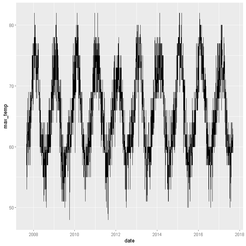

The temperatures are in farenheit. Yup, summer falls in Dec-Jan-Feb.

Import hourly weather data

The hourly data is a little different. The date information is spread over three columns year, month and mday, so we’ll need to use make_date() to combine them.

akl_hourly_raw <- read_csv("datasets/akl_weather_hourly_2016.csv")
head(akl_hourly_raw)

Parsed with column specification:
cols(
  year = col_double(),
  month = col_double(),
  mday = col_double(),
  time = col_time(format = ""),
  temperature = col_double(),
  weather = col_character(),
  conditions = col_character(),
  events = col_character(),
  humidity = col_double(),
  date_utc = col_datetime(format = "")
)

year	month	mday	time	temperature	weather	conditions	events	humidity	date_utc
2016	1	1	00:00:00	68	Clear	Clear	NA	68	2015-12-31 11:00:00
2016	1	1	00:30:00	68	Clear	Clear	NA	68	2015-12-31 11:30:00
2016	1	1	01:00:00	68	Clear	Clear	NA	73	2015-12-31 12:00:00
2016	1	1	01:30:00	68	Clear	Clear	NA	68	2015-12-31 12:30:00
2016	1	1	02:00:00	68	Clear	Clear	NA	68	2015-12-31 13:00:00
2016	1	1	02:30:00	68	Clear	Clear	NA	68	2015-12-31 13:30:00

Then the time information is in a separate column again, time. It’s quite common to find date and time split across different variables. One way to construct the datetimes is to paste the date and time together and then parse them.

# Use make_date() to combine year, month and mday 
akl_hourly  <- akl_hourly_raw  %>% 
  mutate(date = make_date(year = year, month = month, day = mday))

# Parse datetime_string 
akl_hourly <- akl_hourly  %>% 
  mutate(
    datetime_string = paste(date, time, sep = "T"),
    datetime = ymd_hms(datetime_string)
  )

# Print date, time and datetime columns of akl_hourly
akl_hourly %>% 
    select(date, time, datetime) %>%
        head()

date	time	datetime
2016-01-01	00:00:00	2016-01-01 00:00:00
2016-01-01	00:30:00	2016-01-01 00:30:00
2016-01-01	01:00:00	2016-01-01 01:00:00
2016-01-01	01:30:00	2016-01-01 01:30:00
2016-01-01	02:00:00	2016-01-01 02:00:00
2016-01-01	02:30:00	2016-01-01 02:30:00

# Plot to check work
akl_hourly %>%
    ggplot(aes(x = datetime, y = temperature)) +
        geom_line()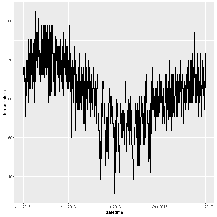

It’s interesting how the day to day variation is about half the size of the yearly variation.

Extracting parts of a datetime

Extracting parts of a datetime

yob = ymd("1997-06-15")
yob

1997-06-15

year(yob)

1997

month(yob)

day(yob)

Extracting parts of a datetime

Function Extracts

year() Year with century

month() Month (1-12)

day() Day of month (1-31)

hour() Hour (0-23)

min() Minute (0-59)

second() Second (0-59)

wday() Weekday (1-7)

Function	Extracts
`year()`	Year with century
`month()`	Month (1-12)
`day()`	Day of month (1-31)
`hour()`	Hour (0-23)
`min()`	Minute (0-59)
`second()`	Second (0-59)
`wday()`	Weekday (1-7)

Setting parts of a datetime

yob

1997-06-15

year(yob) <- 2020

yob

2020-06-15

Other useful functions

Function Extracts

leap_year() In leap year (TRUE or FALSE)

am() In morning (TRUE or FALSE)

pm() In afternoon (TRUE or FALSE)

dst() During daylight savings (TRUE or FALSE)

quarter() Quarter of year (1-4)

semester() Half of year (1-2)

Function	Extracts
`leap_year()`	In leap year (TRUE or FALSE)
`am()`	In morning (TRUE or FALSE)
`pm()`	In afternoon (TRUE or FALSE)
`dst()`	During daylight savings (TRUE or FALSE)
`quarter()`	Quarter of year (1-4)
`semester()`	Half of year (1-2)

# Examine the head() of release_time
head(releases$datetime)

[1] "1997-12-04 08:47:58 UTC" "1997-12-21 13:09:22 UTC"
[3] "1998-01-10 00:31:55 UTC" "1998-03-14 19:25:55 UTC"
[5] "1998-05-02 07:58:17 UTC" "1998-06-14 12:56:20 UTC"

# Examine the head() of the months of release_time
head(month(releases$datetime))

# Extract the month of releases 
month(releases$datetime) %>% table()

.
 1  2  3  4  5  6  7  8  9 10 11 12 
 5  6  8 18  5 16  4  7  2 15  6 13

# Extract the year of releases
year(releases$datetime) %>% table()

.
1997 1998 1999 2000 2001 2002 2003 2004 2005 2006 2007 2008 2009 2010 2011 2012 
   2   10    9    6    6    5    5    4    4    4    4    6    5    4    6    4 
2013 2014 2015 2016 2017 
   4    4    5    5    3

# How often is the hour before 12 (noon)?
mean(hour(releases$datetime) < 12)

0.752380952380952

# How often is the release in am?
mean(am(releases$datetime))

0.752380952380952

R versions have historically been released most in April, June, October and December, 1998 saw 10 releases and about 75% of releases happen in the morning (at least according to UTC).

Adding useful labels

Sometimes it’s nicer (especially for plotting or tables) to have named months. Both the month() and wday() (day of the week) functions have additional arguments label and abbr to achieve just that. Set label = TRUE to have the output labelled with month (or weekday) names, and abbr = FALSE for those names to be written in full rather than abbreviated.

# Use wday() to tabulate release by day of the week
wday(releases$datetime) %>% table()

.
 1  2  3  4  5  6  7 
 3 29  9 12 18 31  3

# Add label = TRUE to make table more readable
wday(releases$datetime, label=TRUE) %>% table()

.
Sun Mon Tue Wed Thu Fri Sat 
  3  29   9  12  18  31   3

# Create column wday to hold labelled week days
releases$wday <- wday(releases$datetime, label=T)

# Plot barchart of weekday by type of release
releases %>%
    ggplot(aes(wday)) +
        geom_bar() +
        facet_wrap(~ type, ncol = 1, scale = "free_y")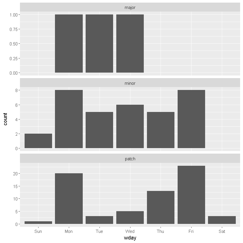

Looks like not too many releases occur on the weekends, and there is quite a different weekday pattern between minor and patch releases.

Extracting for plotting

Extracting components from a datetime is particularly useful when exploring data. Earlier we imported daily data for weather in Auckland, and created a time series plot of ten years of daily maximum temperature. While that plot gives a good overview of the whole ten years, it’s hard to see the annual pattern.

We’ll use components of the dates to help explore the pattern of maximum temperature over the year. The first step is to create some new columns to hold the extracted pieces, then we’ll use them in a couple of plots.

# Add columns for year, yday and month
akl_daily <- akl_daily %>%
  mutate(
    year = year(date),
    yday = yday(date),
    month = month(date, label=T))

# Plot max_temp by yday for all years
akl_daily %>%
    ggplot(aes(x = yday, y = max_temp)) +
    geom_line(aes(group = year), alpha = 0.5)

Warning message:
"Removed 1 row(s) containing missing values (geom_path)."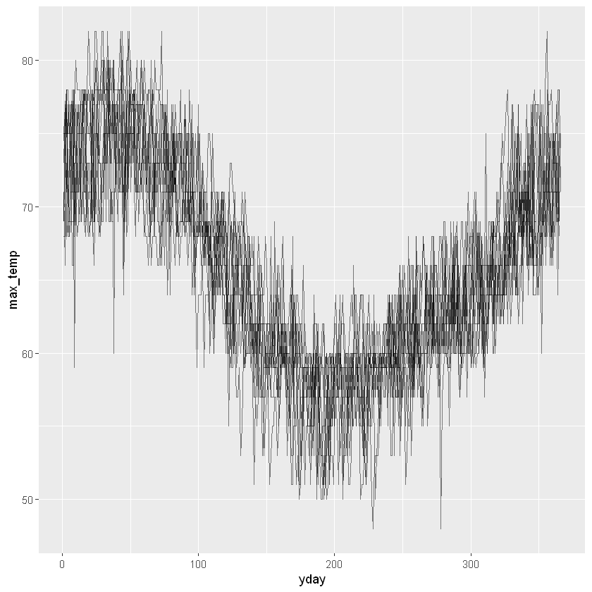

# Examine distribution of max_temp by month
akl_daily %>%
    ggplot(aes(x = max_temp, y = month, height = ..density..)) +
    geom_density_ridges(stat = "density")

Warning message:
"Removed 10 rows containing non-finite values (stat_density)."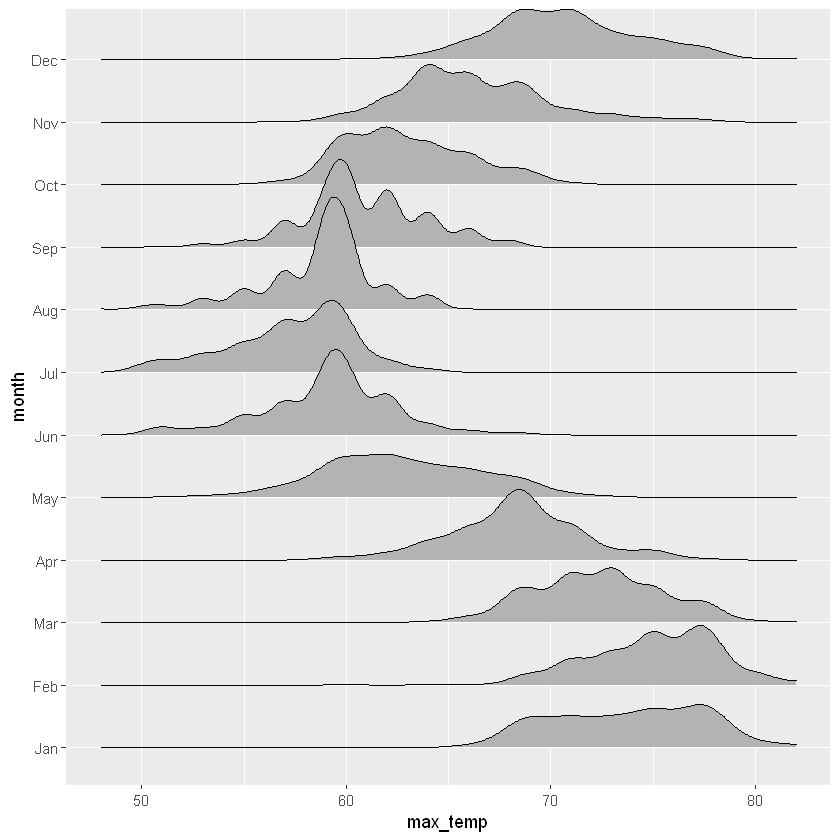

Both plots give a great view into both the expected temperatures and how much they vary. Looks like Jan, Feb and Mar are great months to visit if you want warm temperatures. Did you notice the warning messages? These are a consequence of some missing values in the max_temp column. They are a reminder to think carefully about what you might miss by ignoring missing values.

Extracting for filtering and summarizing

Another reason to extract components is to help with filtering observations or creating summaries. For example, if you are only interested in observations made on weekdays (i.e. not on weekends) you could extract the weekdays then filter out weekends, e.g. wday(date) %in% 2:6.

We saw that January, February and March were great times to visit Auckland for warm temperatures, but will you need a raincoat?

We’ll use the hourly data to calculate how many days in each month there was any rain during the day.

# Create new columns hour, month and rainy
akl_hourly <- akl_hourly %>%
  mutate(
    hour = hour(datetime),
    month = month(datetime, label=T),
    rainy = weather == "Precipitation"
  )

# Filter for hours between 8am and 10pm (inclusive)
akl_day <- akl_hourly %>% 
  filter(hour>=8, hour<=22)

# Summarise for each date if there is any rain
rainy_days <- akl_day %>% 
  group_by(month, date) %>%
  summarise(
    any_rain = any(rainy)
  )

# Summarise for each month, the number of days with rain
rainy_days<- rainy_days %>% 
    summarise(
        days_rainy = sum(any_rain)
    )
rainy_days

`summarise()` regrouping output by 'month' (override with `.groups` argument)
`summarise()` ungrouping output (override with `.groups` argument)

month	days_rainy
Jan	15
Feb	13
Mar	12
Apr	15
May	21
Jun	19
Jul	22
Aug	16
Sep	25
Oct	20
Nov	19
Dec	11

At least in 2016, it looks like you’ll still need to pack a raincoat if you visit in Jan, Feb or March. Months of course are different lengths so we should really correct for that, take a look at days_in_month() for helping with that.

Rounding datetimes

Rounding versus extracting

release_time = releases$datetime
head(release_time)

[1] "1997-12-04 08:47:58 UTC" "1997-12-21 13:09:22 UTC"
[3] "1998-01-10 00:31:55 UTC" "1998-03-14 19:25:55 UTC"
[5] "1998-05-02 07:58:17 UTC" "1998-06-14 12:56:20 UTC"

release_time %>%
    head() %>%
        hour()

release_time %>%
    head() %>%
        floor_date(unit="hour")

[1] "1997-12-04 08:00:00 UTC" "1997-12-21 13:00:00 UTC"
[3] "1998-01-10 00:00:00 UTC" "1998-03-14 19:00:00 UTC"
[5] "1998-05-02 07:00:00 UTC" "1998-06-14 12:00:00 UTC"

Rounding in lubridate

round_date() - round to nearest

ceiling_date() - round up

floor_date() - round to down

Possible values of unit:

"second", "minute", "hour", "day", "week", "month", "bimonth", "quarter", "halfyear", or "year".

Or multiples, e.g "2 years", "5 minutes"

r_3_4_1 <- ymd_hms("2016-05-03 07:13:28 UTC")

# Round down to day
floor_date(r_3_4_1, unit = "day")

[1] "2016-05-03 UTC"

# Round to nearest 5 minutes
round_date(r_3_4_1, unit = "5 minutes")

[1] "2016-05-03 07:15:00 UTC"

# Round up to week 
ceiling_date(r_3_4_1, unit = "week")

[1] "2016-05-08 UTC"

# Subtract r_3_4_1 rounded down to day
r_3_4_1 - floor_date(r_3_4_1, unit = "day")

Time difference of 7.224444 hours

That last technique of subtracting a rounded datetime from an unrounded one is a really useful trick to remember.

Rounding with the weather data

When is rounding useful? In a lot of the same situations extracting date components is useful. The advantage of rounding over extracting is that it maintains the context of the unit. For example, extracting the hour gives you the hour the datetime occurred, but you lose the day that hour occurred on (unless you extract that too), on the other hand, rounding to the nearest hour maintains the day, month and year.

We’ll explore how many observations per hour there really are in the hourly Auckland weather data.

# Create day_hour, datetime rounded down to hour
akl_hourly <- akl_hourly %>%
  mutate(
    day_hour = floor_date(datetime, unit = "hour")
  )

# Count observations per hour  
akl_hourly %>% 
    count(day_hour) %>%
    head()

day_hour	n
2016-01-01 00:00:00	2
2016-01-01 01:00:00	2
2016-01-01 02:00:00	2
2016-01-01 03:00:00	2
2016-01-01 04:00:00	2
2016-01-01 05:00:00	2

# Find day_hours with n != 2  
akl_hourly %>% 
    count(day_hour) %>%
        filter(n!=2) %>% 
            arrange(desc(n)) %>%
                head()

day_hour	n
2016-04-03 02:00:00	4
2016-09-25 00:00:00	4
2016-06-26 09:00:00	1
2016-09-01 23:00:00	1
2016-09-02 01:00:00	1
2016-09-04 11:00:00	1

Interestingly there are four measurements on 2016-04-03 and 2016-09-25, they happen to be the days Daylight Saving starts and ends.

Arithmetic with Dates and Times

Getting datetimes into R is just the first step. Now we’ve explored how to parse datetimes, we need to explore how to do calculations with them. Here we’ll learn the different ways of representing spans of time with lubridate and how to leverage them to do arithmetic on datetimes. By the end we’ll have calculated how long it’s been since the first man stepped on the moon, generated sequences of dates to help schedule reminders, calculated when an eclipse occurs, and explored the reigns of monarch’s of England (and which ones might have seen Halley’s comet!).

Taking differences of datetimes

Arithmetic for datetimes

datetime_1 - datetime2: Subtraction for time elapsed

datetime_1 + (2 * timespan): Addition and multiplication for generating new datetimes in the past or future

timespan1 / timespan2: Division for change of units

Subtraction of datetimes

last_release_date

2017-06-30

Sys.Date() - last_release_date

Time difference of 1110 days

difftime(Sys.Date(), last_release_date)

Time difference of 1110 days

difftime()

units ="secs","mins","hours","days", or "weeks"

year(yob) <- 1997
yob

1997-06-15

difftime(Sys.Date(), yob, units="weeks")

Time difference of 1204.286 weeks

difftime(Sys.Date(), yob, units="days")

Time difference of 8430 days

difftime(Sys.Date(), yob, units="secs")

Time difference of 728352000 secs

now() and today()

now()

[1] "2020-07-14 09:07:16 EAT"

today()

2020-07-14

str(today())

 Date[1:1], format: "2020-07-14"

How long has it been?

To get finer control over a difference between datetimes use the base function difftime(). For example instead of time1 - time2, we can use difftime(time1, time2).

difftime() takes an argument units which specifies the units for the difference. Your options are "secs", "mins", "hours", "days", or "weeks".

We’ll find the time since the first man stepped on the moon.

# The date of landing and moment of step
date_landing <- mdy("July 20, 1969")
moment_step <- mdy_hms("July 20, 1969, 02:56:15", tz = "UTC")

# How many days since the first man on the moon?
difftime(today(), date_landing, units = "days")

Time difference of 18622 days

# How many seconds since the first man on the moon?
difftime(now(), moment_step, units="secs")

Time difference of 1608952266 secs

How many seconds are in a day?

How many seconds are in a day? There are 24 hours in a day, 60 minutes in an hour, and 60 seconds in a minute, so there should be 246060 = 86400 seconds, right?

Not always! We’ll see a counter example.

# Three dates
mar_11 <- ymd_hms("2017-03-11 12:00:00", 
  tz = "America/Los_Angeles")
mar_12 <- ymd_hms("2017-03-12 12:00:00", 
  tz = "America/Los_Angeles")
mar_13 <- ymd_hms("2017-03-13 12:00:00", 
  tz = "America/Los_Angeles")

# Difference between mar_13 and mar_12 in seconds
difftime(mar_13, mar_12, units = "secs")

Time difference of 86400 secs

# Difference between mar_12 and mar_11 in seconds
difftime(mar_12, mar_11, units = "secs")

Time difference of 82800 secs

Why would a day only have 82800 seconds? At 2am on Mar 12th 2017, Daylight Savings started in the Pacific timezone. That means a whole hour of seconds gets skipped between noon on the 11th and noon on the 12th.

Time spans.

Time spans in lubridate

period Duration

Human concept of a timespan Stopwatch concept of a time span

datetime + period of oneday = same time on the next date datetime + duration of oneday = datetime + 86400seconds

variable length fixed number of seconds

period	Duration
Human concept of a timespan	Stopwatch concept of a time span
`datetime + period` of `oneday` = same time on the next date	datetime + duration of oneday = datetime + 86400seconds
variable length	fixed number of seconds

Creating a time span

days()

1d 0H 0M 0S

days(x=2)

2d 0H 0M 0S

ddays(2)

172800s (~2 days)

Arithmetic with time spans

2 * days()

2d 0H 0M 0S

days() + days()

2d 0H 0M 0S

ymd("2020-07-13") + days()

2020-07-14

Functions to create time spans

Time span Duration Period

Seconds dseconds() seconds()

Minutes dminutes() minutes()

Hours dhours() hours()

Days ddays() days()

Weeks dweeks() weeks()

Months - months()

Years dyears() years()

Time span	Duration	Period
Seconds	`dseconds()`	`seconds()`
Minutes	`dminutes()`	`minutes()`
Hours	`dhours()`	`hours()`
Days	`ddays()`	`days()`
Weeks	`dweeks()`	`weeks()`
Months	-	`months()`
Years	`dyears()`	`years()`

ddays()

86400s (~1 days)

Adding or subtracting a time span to a datetime

A common use of time spans is to add or subtract them from a moment in time. For, example to calculate the time one day in the future from mar_11, you could do either of:

mar_11+days()

[1] "2017-03-12 12:00:00 PDT"

mar_11+ddays()

[1] "2017-03-12 13:00:00 PDT"

But which one is the right one? It depends on your intent. If you want to account for the fact that time units, in this case days, have different lengths (i.e. due to daylight savings), you want a period days(). If you want the time 86400 seconds in the future you use a duration ddays().

We’ll add and subtract timespans from dates and datetimes.

# Add a period of one week to mon_2pm
mon_2pm <- dmy_hm("27 Aug 2018 14:00")
mon_2pm + weeks()

[1] "2018-09-03 14:00:00 UTC"

# Add a duration of 81 hours to tue_9am
tue_9am <- dmy_hm("28 Aug 2018 9:00")
tue_9am + dhours(81)

[1] "2018-08-31 18:00:00 UTC"

# Subtract a period of five years from today()
today() - years(5)

2015-07-14

# Subtract a duration of five years from today()
today() - dyears(5)

[1] "2015-07-14 18:00:00 UTC"

Why did subtracting a duration of five years from today, give a different answer to subtracting a period of five years? Periods know about leap years, and since five years ago includes at least one leap year, the period of five years is longer than the duration of 365*5 days.

Note

when dealing with human interpretaions of dates and time you want to use periods.

Arithmetic with timespans

You can add and subtract timespans to create different length timespans, and even multiply them by numbers. For example, to create a duration of three days and three hours you could do:

ddays(3) + dhours(3)

270000s (~3.12 days)

3*ddays(1) + 3*dhours(1)

270000s (~3.12 days)

or even

3*(ddays(1) + dhours(1))

270000s (~3.12 days)

There was an eclipse over North America on 2017-08-21 at 18:26:40. It’s possible to predict the next eclipse with similar geometry by calculating the time and date one Saros in the future. A Saros is a length of time that corresponds to 223 Synodic months, a Synodic month being the period of the Moon’s phases, a duration of 29 days, 12 hours, 44 minutes and 3 seconds.

# Time of North American Eclipse 2017
eclipse_2017 <- ymd_hms("2017-08-21 18:26:40")

# Duration of 29 days, 12 hours, 44 mins and 3 secs
synodic <- ddays(29) + dhours(12) + dminutes(44) + dseconds(3)

# 223 synodic months
saros <- 223 * synodic

# Add saros to eclipse_2017
saros + eclipse_2017

[1] "2035-09-02 02:09:49 UTC"

2035 is a long way away for an eclipse, but luckily there are eclipses on different Saros cycles, so you can see one much sooner.

Generating sequences of datetimes

By combining addition and multiplication with sequences you can generate sequences of datetimes. For example, you can generate a sequence of periods from 1 day up to 10 days with,

1:10 * days()

1d 0H 0M 0S
2d 0H 0M 0S
3d 0H 0M 0S
4d 0H 0M 0S
5d 0H 0M 0S
6d 0H 0M 0S
7d 0H 0M 0S
8d 0H 0M 0S
9d 0H 0M 0S
10d 0H 0M 0S

Then by adding this sequence to a specific datetime, you can construct a sequence of datetimes from 1 day up to 10 days into the future

today() + 1:10 * days()

2020-07-15
2020-07-16
2020-07-17
2020-07-18
2020-07-19
2020-07-20
2020-07-21
2020-07-22
2020-07-23
2020-07-24

We had a meeting this morning at 8am and we’d like to have that meeting at the same time and day every two weeks for a year.

# Add a period of 8 hours to today
today_8am <- today() + hours(8)

# Sequence of two weeks from 1 to 26
every_two_weeks <- 1:26 * weeks()

# Create datetime for every two weeks for a year

every_two_weeks + today_8am

 [1] "2020-07-21 08:00:00 UTC" "2020-07-28 08:00:00 UTC"
 [3] "2020-08-04 08:00:00 UTC" "2020-08-11 08:00:00 UTC"
 [5] "2020-08-18 08:00:00 UTC" "2020-08-25 08:00:00 UTC"
 [7] "2020-09-01 08:00:00 UTC" "2020-09-08 08:00:00 UTC"
 [9] "2020-09-15 08:00:00 UTC" "2020-09-22 08:00:00 UTC"
[11] "2020-09-29 08:00:00 UTC" "2020-10-06 08:00:00 UTC"
[13] "2020-10-13 08:00:00 UTC" "2020-10-20 08:00:00 UTC"
[15] "2020-10-27 08:00:00 UTC" "2020-11-03 08:00:00 UTC"
[17] "2020-11-10 08:00:00 UTC" "2020-11-17 08:00:00 UTC"
[19] "2020-11-24 08:00:00 UTC" "2020-12-01 08:00:00 UTC"
[21] "2020-12-08 08:00:00 UTC" "2020-12-15 08:00:00 UTC"
[23] "2020-12-22 08:00:00 UTC" "2020-12-29 08:00:00 UTC"
[25] "2021-01-05 08:00:00 UTC" "2021-01-12 08:00:00 UTC"

The tricky thing about months

What should ymd(“2018-01-31”) + months(1) return?

ymd("2018-01-31") + months(1)

<NA>

In general lubridate returns the same day of the month in the next month, but since the 31st of February doesn’t exist lubridate returns a missing value, NA.

There are alternative addition and subtraction operators: %m+% and %m-% that have different behavior. Rather than returning an NA for a non-existent date, they roll back to the last existing date

ymd("2018-01-31") %m+% months(1)

2018-02-28

jan_31 = ymd("2020-01-31")
# A sequence of 1 to 12 periods of 1 month
month_seq <- 1:12 * months(1)

# Add 1 to 12 months to jan_31
month_seq + jan_31

<NA>
2020-03-31
<NA>
2020-05-31
<NA>
2020-07-31
2020-08-31
<NA>
2020-10-31
<NA>
2020-12-31
2021-01-31

# Replace + with %m+%
month_seq %m+% jan_31

2020-02-29
2020-03-31
2020-04-30
2020-05-31
2020-06-30
2020-07-31
2020-08-31
2020-09-30
2020-10-31
2020-11-30
2020-12-31
2021-01-31

# Replace + with %m-%
jan_31 %m-% month_seq

2019-12-31
2019-11-30
2019-10-31
2019-09-30
2019-08-31
2019-07-31
2019-06-30
2019-05-31
2019-04-30
2019-03-31
2019-02-28
2019-01-31

Warning

use these operators with caution, unlike + and -, you might not get x back from x %m+% months(1) %m-% months(1). If you’d prefer that the date was rolled forward check out add_with_rollback() which has roll_to_first argument.

Intervals

Creating intervals

datetime1%--%datetime2,or

interval(datetime1, datetime2)

yob %--% today()

1997-06-15 UTC--2020-07-14 UTC

interval(yob, today())

1997-06-15 UTC--2020-07-14 UTC

Operating on an interval

yob_interval = interval(yob, today())
int_start(yob_interval)

[1] "1997-06-15 UTC"

int_end(yob_interval)

[1] "2020-07-14 UTC"

Operating on an interval

int_length(yob_interval)

728352000

as.period(yob_interval)

23y 0m 29d 0H 0M 0S

as.duration(yob_interval)

728352000s (~23.08 years)

Comparing intervals

enter_mmu <- ymd("2017-07-30")
enter_mmu %within% yob_interval

TRUE

been_mmu <- ymd("2017-07-30") %--% today()

int_overlaps(been_mmu, yob_interval)

TRUE

Which kind of time span?

Use:

Intervals when you have a start and end

Periods when you are interested in human units

Durations if you are interested in seconds elapsed

Monarchs of England {% fn 2 %}
Halley’s cometHalley’scomet:{% fn 3 %}

Examining intervals. Reigns of kings and queens

# Print monarchs
monarchs

# Create an interval for reign
monarchs <- monarchs %>%
  mutate(reign = from %--% to) 

# Find the length of reign, and arrange
monarchs %>%
  mutate(length = int_length(reign)) %>% 
  arrange(desc(length)) %>%
  select(name, length, dominion)

The current queen, Elizabeth II, has ruled for 2070144000 seconds…we’ll see a better way to display the length later. If you know your British monarchs, you might notice George III doesn’t appear in the the top 5. In this data, his reign is spread over two rows for U.K. And Great Britain and you would need to add their lengths to see his total reign.

Comparing intervals and datetimes

A common task with intervals is to ask if a certain time is inside the interval or whether it overlaps with another interval.

The operator %within% tests if the datetime (or interval) on the left hand side is within the interval of the right hand side. For example, if y2001 is the interval covering the year 2001,

y2001 <- ymd("2001-01-01") %--% ymd("2001-12-31")
ymd("2001-03-30") %within% y2001

TRUE

ymd("2002-03-30") %within% y2001

FALSE

int_overlaps() performs a similar test, but will return true if two intervals overlap at all.

# Print halleys
halleys

# New column for interval from start to end date
halleys <- halleys %>% 
  mutate(visible = interval(start_date, end_date))

# The visitation of 1066
halleys_1066 <- halleys[14, ] 

# Monarchs in power on perihelion date
monarchs %>% 
  filter(halleys_1066$perihelion_date %within%reign) %>%
  select(name, from, to, dominion)

# Monarchs whose reign overlaps visible time
monarchs %>% 
  filter(int_overlaps(halleys_1066$visible,reign)) %>%
  select(name, from, to, dominion)

Looks like the Kings of England Edward the Confessor and Harold II would have been able to see the comet. It may have been a bad omen, neither were in power by 1067.

Converting to durations and periods

Intervals are the most specific way to represent a span of time since they retain information about the exact start and end moments. They can be converted to periods and durations exactly: it’s possible to calculate both the exact number of seconds elapsed between the start and end date, as well as the perceived change in clock time

# New columns for duration and period
monarchs <- monarchs %>%
  mutate(
    duration = as.duration(reign),
    period = as.period(reign)) 
    
# Examine results    
monarchs %>%
  select(name, duration, period)

Problems in practice

You now know most of what you need to tackle data that includes dates and times, but there are a few other problems we might encounter. We’ll explore a little more about these problems by returning to some of the earlier data sets and explore how to handle time zones, deal with times when you don’t care about dates, parse dates quickly, and output dates and times.

Time zones

Sys.timezone()

'Africa/Nairobi'

IANA Timezones

OlsonNames() %>%
    head(10)

'Africa/Abidjan'
'Africa/Accra'
'Africa/Addis_Ababa'
'Africa/Algiers'
'Africa/Asmara'
'Africa/Asmera'
'Africa/Bamako'
'Africa/Bangui'
'Africa/Banjul'
'Africa/Bissau'

length(OlsonNames())

593

Setting and extracting

mar_11

[1] "2017-03-11 12:00:00 PST"

tz(mar_11)

'America/Los_Angeles'

Manipulating timezones

force_tz() - change thetimezone without changing the clock time

with_tz() - view the sameinstant in a different timezone

with_tz(mar_11, tzone="Africa/Nairobi")

[1] "2017-03-11 23:00:00 EAT"

force_tz(mar_11, tzone="Africa/Nairobi")

[1] "2017-03-11 12:00:00 EAT"

Setting the timezone

If you import a datetime and it has the wrong timezone, you can set it with force_tz(). Pass in the datetime as the first argument and the appropriate timezone to the tzone argument. Remember the timezone needs to be one from OlsonNames().

I wanted to watch New Zealand in the Women’s World Cup Soccer games in 2015, but the times listed on the FIFA website were all in times local to the venues. We’ll set the timezones, then figure out what time I needed to tune in to watch them.

# Game2: CAN vs NZL in Edmonton
game2 <- mdy_hm("June 11 2015 19:00")

# Game3: CHN vs NZL in Winnipeg
game3 <- mdy_hm("June 15 2015 18:30")

# Set the timezone to "America/Edmonton"
game2_local <- force_tz(game2, tzone = "America/Edmonton")
game2_local

[1] "2015-06-11 19:00:00 MDT"

# Set the timezone to "America/Winnipeg"
game3_local <- force_tz(game3, tzone = "America/Winnipeg")
game3_local

[1] "2015-06-15 18:30:00 CDT"

# How long does the team have to rest?
as.period(interval(game2_local, game3_local))

3d 22H 30M 0S

Edmonton and Winnipeg are in different timezones, so even though the start times of the games only look 30 minutes apart, they are in fact 1 hour and 30 minutes apart, and the team only has 3 days, 22 hours and 30 minutes to prepare.

Viewing in a timezone

To view a datetime in another timezone use with_tz(). The syntax of with_tz() is the same as force_tz(), passing a datetime and set the tzone argument to the desired timezone. Unlike force_tz(), with_tz() isn’t changing the underlying moment of time, just how it is displayed.

# What time is game2_local in NZ?
with_tz(game2_local, tzone = "Pacific/Auckland")

[1] "2015-06-12 13:00:00 NZST"

# What time is game2_local in Corvallis, Oregon?
with_tz(game2_local, tzone = "America/Los_Angeles")

[1] "2015-06-11 18:00:00 PDT"

# What time is game3_local in NZ?
with_tz(game3_local, tzone="Pacific/Auckland")

[1] "2015-06-16 11:30:00 NZST"

Timezones in the weather data

head(akl_hourly)

year	month	mday	time	temperature	weather	conditions	events	humidity	date_utc	date	datetime_string	datetime	hour	rainy	day_hour
2016	Jan	1	00:00:00	68	Clear	Clear	NA	68	2015-12-31 11:00:00	2016-01-01	2016-01-01T00:00:00	2016-01-01 00:00:00	0	FALSE	2016-01-01 00:00:00
2016	Jan	1	00:30:00	68	Clear	Clear	NA	68	2015-12-31 11:30:00	2016-01-01	2016-01-01T00:30:00	2016-01-01 00:30:00	0	FALSE	2016-01-01 00:00:00
2016	Jan	1	01:00:00	68	Clear	Clear	NA	73	2015-12-31 12:00:00	2016-01-01	2016-01-01T01:00:00	2016-01-01 01:00:00	1	FALSE	2016-01-01 01:00:00
2016	Jan	1	01:30:00	68	Clear	Clear	NA	68	2015-12-31 12:30:00	2016-01-01	2016-01-01T01:30:00	2016-01-01 01:30:00	1	FALSE	2016-01-01 01:00:00
2016	Jan	1	02:00:00	68	Clear	Clear	NA	68	2015-12-31 13:00:00	2016-01-01	2016-01-01T02:00:00	2016-01-01 02:00:00	2	FALSE	2016-01-01 02:00:00
2016	Jan	1	02:30:00	68	Clear	Clear	NA	68	2015-12-31 13:30:00	2016-01-01	2016-01-01T02:30:00	2016-01-01 02:30:00	2	FALSE	2016-01-01 02:00:00

The datetime column we created represented local time in Auckland, NZ. I suspect this additional column, date_utc represents the observation time in UTC (the name seems a big clue). But does it really?

# Examine datetime and date_utc columns
head(akl_hourly$datetime)

[1] "2016-01-01 00:00:00 UTC" "2016-01-01 00:30:00 UTC"
[3] "2016-01-01 01:00:00 UTC" "2016-01-01 01:30:00 UTC"
[5] "2016-01-01 02:00:00 UTC" "2016-01-01 02:30:00 UTC"

head(akl_hourly$date_utc)

[1] "2015-12-31 11:00:00 UTC" "2015-12-31 11:30:00 UTC"
[3] "2015-12-31 12:00:00 UTC" "2015-12-31 12:30:00 UTC"
[5] "2015-12-31 13:00:00 UTC" "2015-12-31 13:30:00 UTC"

# Force datetime to Pacific/Auckland
akl_hourly <- akl_hourly %>%
  mutate(
    datetime = force_tz(datetime, tzone = "Pacific/Auckland"))

# Reexamine datetime
head(akl_hourly$datetime)

[1] "2016-01-01 00:00:00 NZDT" "2016-01-01 00:30:00 NZDT"
[3] "2016-01-01 01:00:00 NZDT" "2016-01-01 01:30:00 NZDT"
[5] "2016-01-01 02:00:00 NZDT" "2016-01-01 02:30:00 NZDT"

# Are datetime and date_utc the same moments
table(akl_hourly$datetime - akl_hourly$date_utc)


-82800      0   3600 
     2  17450      2

Looks like for 17,450 rows datetime and date_utc describe the same moment, but for 4 rows they are different. Can you guess which? Yup, the times where DST kicks in.

Times without dates

# Examine structure of time column
str(akl_hourly$time)

 'hms' num [1:17454] 00:00:00 00:30:00 01:00:00 01:30:00 ...
 - attr(*, "units")= chr "secs"

# Examine head of time column
head(akl_hourly$time)

00:00:00
00:30:00
01:00:00
01:30:00
02:00:00
02:30:00

# A plot using just time
akl_hourly %>% 
    ggplot(aes(x = time, y = temperature)) +
    geom_line(aes(group = make_date(year, month, mday)), alpha = 0.2)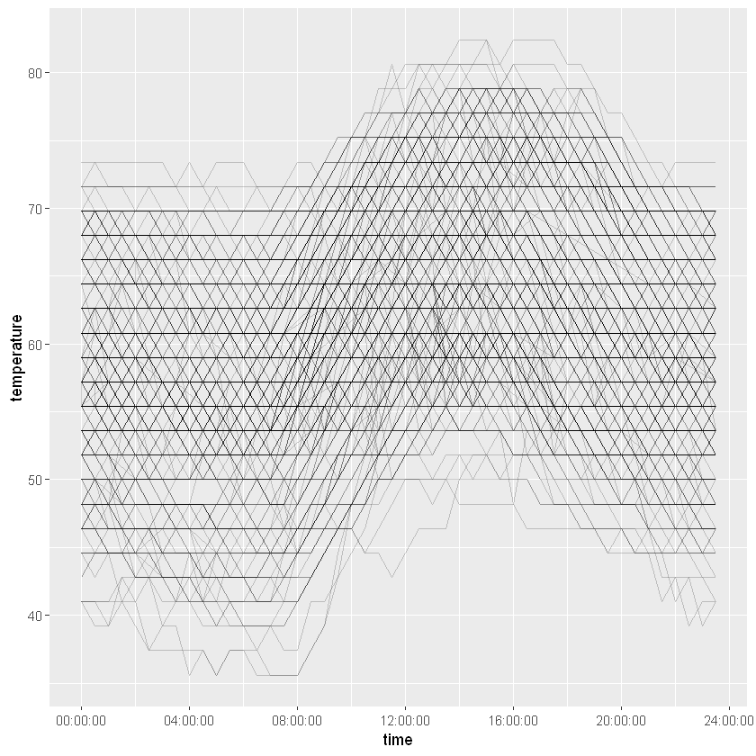

Using time without date is a great way to examine daily patterns.

More on importing and exporting datetimes

Fast parsing

parse_date_time() can be slow because it’s designed to be forgiving and flexible.

fastPOSIXct("1997-06-16")

[1] "1997-06-16 03:00:00 EAT"

fast_strptime()

yob_str <- "1997-06-15"
parse_date_time(yob_str, order="ymd")

[1] "1997-06-15 UTC"

fast_strptime(yob_str, format = "%Y-%m-%d")

[1] "1997-06-15 UTC"

Exporting datetimes

akl_hourly %>%
    select(datetime) %>%
    write_csv("datasets/tmp.csv")

Formatting datetimes

yob_stamp <- stamp("Sunday June 15 1997")

Multiple formats matched: "%A %B %d %Y"(1), "Sunday %Om %d %Y"(1), "Sunday %B %d %Y"(1), "%A %Om %d %Y"(0)
Using: "%A %B %d %Y"

yob_stamp(ymd("1997-06-15"))

'Sunday June 15 1997'

yob_stamp

function (x, locale = "English_United States.1252") 
{
    {
        old_lc_time <- Sys.getlocale("LC_TIME")
        if (old_lc_time != locale) {
            on.exit(Sys.setlocale("LC_TIME", old_lc_time))
            Sys.setlocale("LC_TIME", locale)
        }
    }
    format(x, format = "%A %B %d %Y")
}

Fast parsing with fasttime

The fasttime package provides a single function fastPOSIXct(), designed to read in datetimes formatted according to ISO 8601. Because it only reads in one format, and doesn’t have to guess a format, it is really fast!

We’ll see how fast by comparing how fast it reads in the dates from the Auckland hourly weather data (over 17,000 dates) to lubridates ymd_hms().

# Examine structure of dates
str(akl_hourly$datetime_string)

 chr [1:17454] "2016-01-01T00:00:00" "2016-01-01T00:30:00" ...

# Use fastPOSIXct() to parse dates
fastPOSIXct(akl_hourly$datetime_string) %>% str()

 POSIXct[1:17454], format: "2016-01-01 03:00:00" "2016-01-01 03:30:00" "2016-01-01 04:00:00" ...

# Compare speed of fastPOSIXct() to ymd_hms()
microbenchmark(
  ymd_hms = ymd_hms(akl_hourly$datetime_string),
  fasttime = fastPOSIXct(akl_hourly$datetime_string),
  times = 20)

expr	time
fasttime	2455100
ymd_hms	30602000
fasttime	2577700
ymd_hms	31090200
fasttime	2762600
fasttime	2779400
fasttime	2796400
fasttime	2786900
ymd_hms	35160800
fasttime	2590900
ymd_hms	32037000
ymd_hms	31251200
ymd_hms	32154400
fasttime	2638200
ymd_hms	32626700
ymd_hms	31518000
fasttime	2517700
ymd_hms	32616500
fasttime	2396500
ymd_hms	33101100
fasttime	2503900
fasttime	2429800
ymd_hms	38136000
ymd_hms	28758100
fasttime	2131100
ymd_hms	26896600
fasttime	2219700
ymd_hms	26722900
ymd_hms	26774200
ymd_hms	28291400
ymd_hms	35462800
ymd_hms	35749400
fasttime	2591500
fasttime	2532400
ymd_hms	32089700
fasttime	2776700
fasttime	2697700
fasttime	2550500
ymd_hms	33218200
fasttime	2475800

fasttime is about 20 times faster than ymd_hms().

Fast parsing with lubridate::fast_strptime

lubridate provides its own fast datetime parser: fast_strptime(). Instead of taking an order argument like parse_date_time() it takes a format argument and the format must comply with the strptime() style.

# Head of dates
head(akl_hourly$datetime_string)

'2016-01-01T00:00:00'
'2016-01-01T00:30:00'
'2016-01-01T01:00:00'
'2016-01-01T01:30:00'
'2016-01-01T02:00:00'
'2016-01-01T02:30:00'

# Parse dates with fast_strptime
fast_strptime(akl_hourly$datetime_string, 
    format = "%Y-%m-%dT%H:%M:%S") %>% str()

 POSIXlt[1:17454], format: "2016-01-01 00:00:00" "2016-01-01 00:30:00" "2016-01-01 01:00:00" ...

# Comparse speed to ymd_hms() and fasttime
microbenchmark(
  ymd_hms = ymd_hms(akl_hourly$datetime_string),
  fasttime = fastPOSIXct(akl_hourly$datetime_string),
  fast_strptime = fast_strptime(akl_hourly$datetime_string, 
    format = "%Y-%m-%dT%H:%M:%S"),
  times = 20)

expr	time
ymd_hms	42620600
ymd_hms	46698300
fast_strptime	3006900
ymd_hms	29005100
ymd_hms	28695300
fasttime	2406000
fasttime	2340100
fasttime	2312100
fasttime	2310500
ymd_hms	31183400
fast_strptime	3118800
fasttime	2325100
ymd_hms	29844300
fast_strptime	3363600
fast_strptime	3071200
ymd_hms	30061000
fasttime	2251400
ymd_hms	36800700
fast_strptime	3555000
ymd_hms	34068400
fasttime	2512300
fast_strptime	3111700
fast_strptime	3095400
fasttime	2264900
fast_strptime	3090500
ymd_hms	36769000
ymd_hms	27374000
fast_strptime	2777400
ymd_hms	27985100
fasttime	2200400
fasttime	1994100
fast_strptime	2602500
fast_strptime	2617500
ymd_hms	26029600
ymd_hms	26985200
fast_strptime	3005900
fasttime	2201400
fasttime	2131400
ymd_hms	29039200
fasttime	2134500
fasttime	2064700
fast_strptime	2821100
fasttime	2143200
fasttime	2044300
ymd_hms	29941500
fast_strptime	3029800
ymd_hms	41443300
fasttime	2978200
fasttime	3032300
fast_strptime	4292500
fast_strptime	3543800
ymd_hms	35316000
ymd_hms	37035500
fast_strptime	3009300
ymd_hms	27633800
fasttime	2117500
fast_strptime	2832600
fasttime	2035900
fast_strptime	2714100
fast_strptime	2799400

Outputting pretty dates and times

An easy way to output dates is to use the stamp() function in lubridate. stamp() takes a string which should be an example of how the date should be formatted, and returns a function that can be used to format dates.

# Create a stamp based on "Saturday, Jan 1, 2000"
date_stamp <- stamp("Saturday, Jan 1, 2000")

# Print date_stamp
date_stamp

Multiple formats matched: "%A, %b %d, %Y"(1), "Saturday, Jan %Om, %Y"(1), "Saturday, %Om %d, %Y"(1), "Saturday, %b %d, %Y"(1), "Saturday, Jan %m, %Y"(1), "%A, Jan %Om, %Y"(0), "%A, %Om %d, %Y"(0), "%A, Jan %m, %Y"(0)
Using: "%A, %b %d, %Y"

function (x, locale = "English_United States.1252") 
{
    {
        old_lc_time <- Sys.getlocale("LC_TIME")
        if (old_lc_time != locale) {
            on.exit(Sys.setlocale("LC_TIME", old_lc_time))
            Sys.setlocale("LC_TIME", locale)
        }
    }
    format(x, format = "%A, %b %d, %Y")
}

# Call date_stamp on today()
date_stamp(today())

'Tuesday, Jul 14, 2020'

# Create and call a stamp based on "12/31/1999"
stamp("12/31/1999")(today())

Multiple formats matched: "%Om/%d/%Y"(1), "%m/%d/%Y"(1)
Using: "%Om/%d/%Y"

'07/14/2020'

finished = "I finished 'Dates and Times in R' on Thursday, September 4, 2017!"

# Use string finished for stamp()
stamp(finished)(today())

Multiple formats matched: "I finished 'Dates and Times in R' on %A, %B %d, %Y!"(1), "I finished 'Dates and Times in R' on Thursday, September %Om, %Y!"(1), "I finished 'Dates and Times in R' on Thursday, %Om %d, %Y!"(1), "I finished 'Dates and Times in R' on Thursday, %B %d, %Y!"(1), "I finished 'Dates and Times in R' on Thursday, September %m, %Y!"(1), "I finished 'Dates and Times in R' on %A, September %Om, %Y!"(0), "I finished 'Dates and Times in R' on %A, %Om %d, %Y!"(0), "I finished 'Dates and Times in R' on %A, September %m, %Y!"(0)
Using: "I finished 'Dates and Times in R' on %A, %B %d, %Y!"

'I finished \'Dates and Times in R\' on Tuesday, July 14, 2020!'

Wrapping-up

Chapter 1: base R objects Date, POSIXct
Chapter 2: importing and manipulating datetimes
Chapter 3: arithmetic with datetimes, periods, durations andintervals
Chapter 4: time zones, fast parsing, outputting datetimes

{{‘source: https://xkcd.com/1179’ | fndetail: 1}} {{‘Source: Monarchs of England’ | fndetail: 2 }} {{‘Source: Halley’s cometHalley’scomet:’ | fndetail: 3 }}

Overview

Libraries

Dates and Times in R

Introduction to dates

Dates

The global standard numeric date format

ISO 8601 YYYY-MM-DD

Specifying dates

Automatic import

Why use dates?

Dates act like numbers

Plotting with dates

R releases

Plotting

Arithmetic and logical operators

What about times?

ISO 8601

Datetimes in R

Timezones

Datetimes behave nicely too

Getting datetimes into R

Datetimes behave nicely too

Why lubridate?

lubridate

Parsing a wide range of formats

Manipulating datetimes

Other lubridate features

Parsing and Manipulating Dates and Times with lubridate

Parsing dates with lubridate

ymd()

Friends of ymd()

Formatting characters

Selecting the right parsing function

Specifying an order with parse_date_time()

Weather in Auckland

make_date(year, month, day)

dplyr Review

Import daily weather data

Import hourly weather data

Extracting parts of a datetime

Extracting parts of a datetime

Extracting parts of a datetime

Setting parts of a datetime

Other useful functions

Adding useful labels

Extracting for plotting

Extracting for filtering and summarizing

Rounding datetimes

Rounding versus extracting

Rounding in lubridate

Rounding with the weather data

Arithmetic with Dates and Times

Taking differences of datetimes

Arithmetic for datetimes

Subtraction of datetimes

difftime()

now() and today()

How long has it been?

How many seconds are in a day?

Time spans.

Time spans in lubridate

Creating a time span

Arithmetic with time spans

Functions to create time spans

Adding or subtracting a time span to a datetime

Arithmetic with timespans

Generating sequences of datetimes

The tricky thing about months

Intervals

Creating intervals

Operating on an interval

Operating on an interval

Comparing intervals

Which kind of time span?

Examining intervals. Reigns of kings and queens

Comparing intervals and datetimes

Converting to durations and periods

Problems in practice

Time zones

IANA Timezones

Specifying an order with `parse_date_time()`